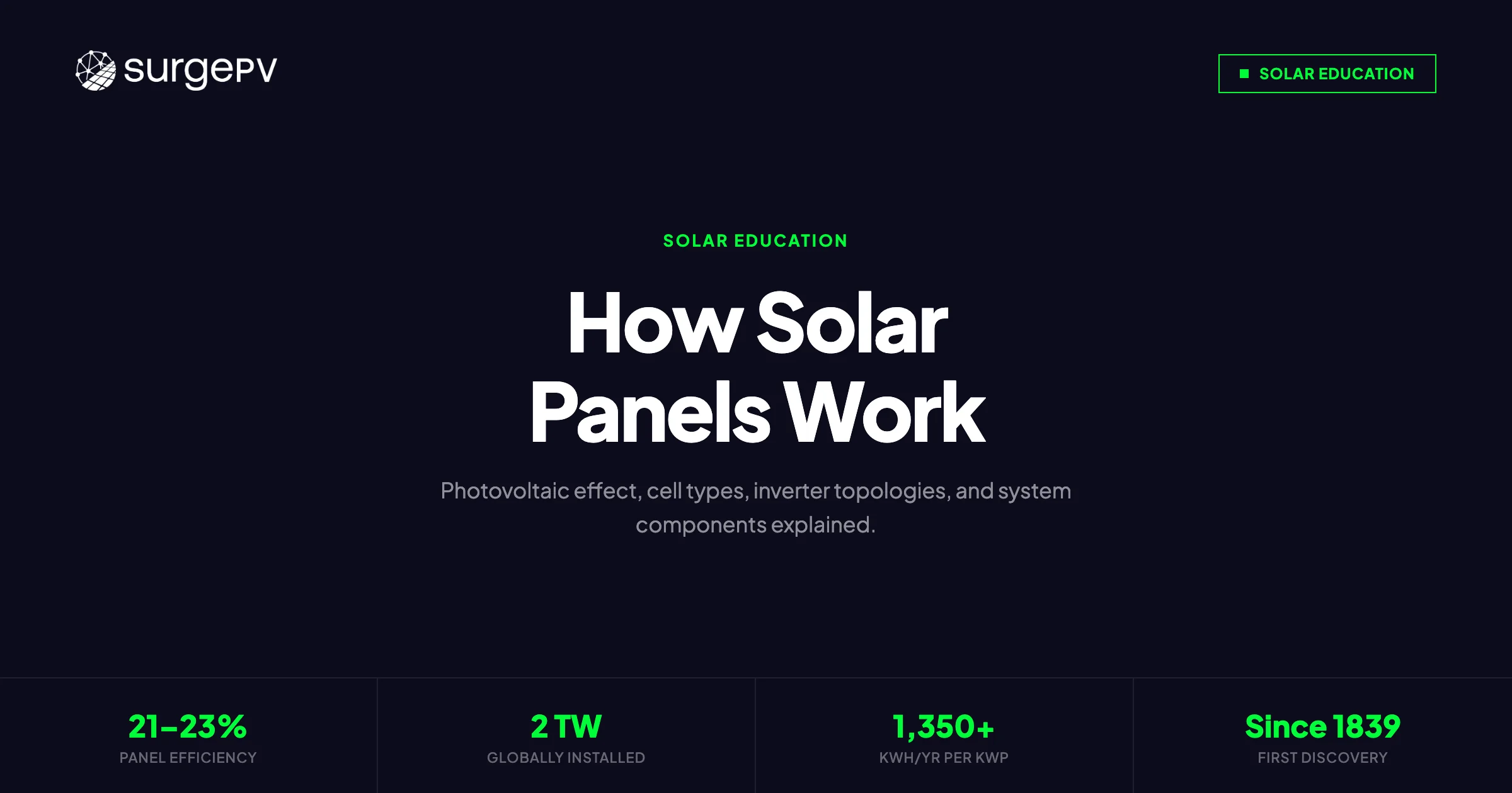
In 1839, Edmond Becquerel noticed that certain materials produced a small electrical current when exposed to light. He had no idea he was describing the operating principle for what would become the largest source of new electricity generation on Earth. By 2026, solar photovoltaic systems have surpassed 2 terawatts of installed capacity globally — more than all nuclear power plants combined — and the physics behind every single panel is still fundamentally the same quantum-mechanical event Becquerel stumbled onto in a Paris laboratory.
Understanding exactly how solar panels work is not just useful trivia for homeowners. For solar installers, designers, and project managers, the physics determines everything: how you string a system, where to place inverters, how much shading matters, why a hot summer day can reduce output despite brilliant sunshine, and how to accurately model annual energy production before a single panel ships to site. This guide builds from the atomic level up to the full system, with every concept connected to real design decisions.
TL;DR — How Solar Panels Work in 2026
Solar panels convert sunlight to electricity via the photovoltaic effect: photons excite electrons in silicon, a p-n junction creates directional current flow, and metal contacts collect DC power. An inverter converts DC to AC for use in buildings. Efficiency of mainstream panels is 21–23% in 2026, with TOPCon cells reaching 24.5%. Temperature, irradiance, and shading all reduce real-world output — which is why accurate modeling matters. A 1 kWp system in a 1,500 kWh/kWp/year location produces roughly 1,350–1,450 kWh annually after system losses.
In this guide:
- How the photovoltaic effect works — from photon to electron to current
- Silicon doping, p-n junctions, and why they create directional flow
- Monocrystalline vs. polycrystalline vs. thin-film: efficiency table and use cases
- Complete system components: panels, inverters, mounting, monitoring
- String vs. microinverter vs. power optimizer topologies
- How irradiance and temperature affect output — real derating curves
- Shading physics, bypass diodes, and string performance impacts
- Energy production calculation: kWp × specific yield × performance ratio
- How design software models all of this — and why it matters for installers
Latest Updates: Solar Panel Technology 2026
The past 24 months have accelerated efficiency, reduced costs, and introduced cell architectures that are now mainstream in new installations.
Efficiency Records — 2025–2026
| Cell Technology | Lab Record (2025–2026) | Commercial Module Range | Key Manufacturers |
|---|---|---|---|
| TOPCon (mono-Si) | 26.1% (cell) | 22.5–24.5% (module) | LONGi, Jinko, Trina, REC |
| HJT (heterojunction) | 26.7% (cell) | 22.0–24.8% (module) | Panasonic, REC Alpha, Huasun |
| Back-Contact HJT | 27.1% (cell) | 23.5–25.0% (module) | SunPower (Maxeon), LONGi |
| Perovskite/Si Tandem | 33.9% (cell, NREL) | 24–26% (early commercial) | Oxford PV, Longi, Tandem.PV |
| CdTe thin-film | 22.1% (cell) | 18.5–20.5% (module) | First Solar |
| CIGS thin-film | 23.6% (cell) | 17.0–20.0% (module) | MiaSolé, Solar Frontier |
Cell records from NREL Best Research-Cell Efficiency Chart, March 2026. Module efficiencies represent commercial volume production, not maximum rated products.
What Changed Since 2024
TOPCon is now the mainstream default. In 2022, PERC (Passivated Emitter and Rear Cell) was the dominant technology. By 2025–2026, nearly all tier-1 manufacturers have transitioned new production lines to TOPCon architecture, which offers 1–1.5 percentage points higher efficiency and better performance in high-temperature and low-light conditions. PERC panels remain available but are now treated as the budget-tier option.
Bifacial modules are standard above 400W. Bifacial panels capture reflected irradiance (albedo) from the ground or roof surface on the rear face of the module. In 2026, bifacial is the default configuration for most commercial and ground-mount projects, adding 5–15% energy yield depending on ground reflectance. Some rooftop applications use bifacial panels with white-membrane roofs to capture rear-side gain.
Perovskite-silicon tandem approaching commercial scale. Oxford PV began volume production of tandem cells above 30% efficiency in 2025. These panels stack a perovskite top cell (optimized for high-energy blue/UV photons) on a silicon bottom cell (capturing red/IR photons), surpassing what any single-junction silicon cell can achieve. Degradation and long-term stability questions remain, but 2026 product warranties are extending to 15 years for tandem commercial modules.
Module wattages crossing 700W for utility scale. Standard residential panels now ship at 400–450W. Commercial and utility modules are now commonly 550–700W per panel, reducing racking, wiring, and labor cost per watt.
Key Takeaway — What 2026 Technology Means for Installers
Switching from PERC to TOPCon for the same roof area increases energy production by 5–8% with no additional structural load. For any new system design, specify TOPCon unless budget constraints require otherwise. The higher upfront module cost is offset within 2–3 years by additional generation revenue.
The Photovoltaic Effect: Step-by-Step Physics
To understand every operational characteristic of a solar system — efficiency, temperature sensitivity, shading behavior, inverter sizing — you need to understand the underlying physics. This is not academic: each physical mechanism maps directly to a design decision or a commissioning check.
Step 1: What a Photon Does to a Silicon Atom
Silicon (Si) is a semiconductor: its electrical conductivity sits between conductors like copper and insulators like glass. In pure crystalline silicon, each atom forms four covalent bonds with neighboring atoms in a rigid lattice. Electrons are bound in these bonds under normal conditions.
When a photon — a quantum of light energy — strikes a silicon crystal, it can transfer its energy to a bound electron. If the photon’s energy exceeds silicon’s bandgap (approximately 1.12 electron-volts), the electron absorbs the photon and is promoted from the valence band to the conduction band. In plain terms: the electron breaks free from its atomic bond and can move through the crystal.
This is the photoelectric effect in a solid — the fundamental event that generates all photovoltaic power.
Two outcomes are possible after this electron excitation:
- The electron recombines with a “hole” (the positive vacancy left when it departed) and the energy is released as heat. This is a loss mechanism.
- The electron is separated and directed toward a contact before recombination occurs. This is useful electricity.
The p-n junction is the mechanism that separates electrons and forces outcome #2.
Step 2: Doping Silicon — Creating p-Type and n-Type Layers
Pure silicon has no excess carriers and produces no net current under light. Solar cells are made from doped silicon:
n-type silicon: Adding phosphorus (5 valence electrons instead of silicon’s 4) introduces extra electrons — called donor electrons — into the lattice. These electrons are not bound to the lattice and are free to move. N-type silicon has an excess of negative carriers (electrons).
p-type silicon: Adding boron (3 valence electrons) creates “holes” in the lattice — positions where an electron is missing. The absence of electrons acts like a positive charge carrier. P-type silicon has an excess of positive carriers (holes).
Neither p-type nor n-type silicon alone produces power. The critical structure is what happens when they are joined.
Step 3: The p-n Junction — Where the Magic Happens
When p-type and n-type silicon are brought into contact, electrons from the n-side diffuse across the junction into the p-side (and holes diffuse in the opposite direction). This diffusion continues until a built-in electric field develops at the junction — oriented from n to p — that opposes further diffusion.
This region of charge separation is called the depletion zone. The built-in electric field acts as a one-way gate:
- Electrons in the n-region that absorb photons near the junction are swept toward the n-contact by the field.
- Holes in the p-region are swept toward the p-contact.
- Photon-generated electron-hole pairs in the depletion zone are immediately separated by the field.
The result is a net flow of electrons through an external circuit from n-contact to p-contact — which is conventional current flowing from p to n. This is direct current (DC).
Step 4: From Junction to Module Output
A single silicon solar cell is approximately 156mm × 156mm (M10 format) or 182mm × 182mm (M10+/G12 format) as of 2026. Under standard test conditions (STC: 1,000 W/m² irradiance, 25°C cell temperature, AM 1.5 solar spectrum), a single silicon cell produces approximately:
- Voltage: 0.55–0.65 V open-circuit (Voc)
- Current: 8–12 A short-circuit (Isc) depending on cell area
- Power: ~4–7W per cell
A standard 60-cell residential panel (now largely replaced by 72-cell and 144 half-cut formats) generates 300–350W. Modern 66-cell or 72-cell panels with M10 or G12 wafers produce 400–450W at STC.
The cells are connected in series within the panel to add voltages while maintaining the same current — this is why a module voltage is roughly 60× the cell voltage (36–44V Vmpp for standard panels).
Step 5: Half-Cut Cell Technology
A major manufacturing shift in the past five years has been the move from full-cell to half-cut cell construction. In half-cut modules:
- Each cell is laser-cut in half, creating cells roughly 78mm × 156mm (for M10 format).
- The resulting smaller cells have lower current per cell (half the original), which reduces resistive losses (I²R losses) by approximately 75%.
- The module is typically wired in two independent sub-strings connected in parallel, so partial shading affects only half the module.
Half-cut cells are now standard across all tier-1 manufacturers and account for the majority of efficiency gains versus equivalent older full-cell designs.
Pro Tip — Cell Temperature vs. Air Temperature
Solar cell temperature is consistently 20–35°C higher than ambient air temperature under full sun. A panel rated at 22% efficiency at 25°C (STC) operates at 45–60°C on a sunny summer day — reducing efficiency by 8–15% from its nameplate rating. Always specify NOCT (Normal Operating Cell Temperature) performance figures when modeling real-world output, not just STC figures.
Monocrystalline vs. Polycrystalline vs. Thin-Film
The cell architecture determines efficiency, cost, temperature behavior, and application suitability. In 2026, the market has largely consolidated around monocrystalline silicon for most applications, but understanding all three types remains relevant for installers who encounter legacy systems or specialized applications.
Technology Comparison — 2026
| Technology | Module Efficiency | Temp Coefficient (Pmax) | Cost/W | Best Application | Degradation/yr |
|---|---|---|---|---|---|
| Monocrystalline PERC | 19.5–21.5% | -0.35 to -0.40%/°C | $0.22–$0.28 | Standard residential/commercial | 0.40–0.50% |
| Monocrystalline TOPCon | 21.5–24.5% | -0.28 to -0.35%/°C | $0.25–0.32 | Premium residential/commercial | 0.30–0.40% |
| Heterojunction (HJT) | 22.0–24.8% | -0.24 to -0.30%/°C | $0.30–0.38 | High-temperature climates, space-constrained roofs | 0.25–0.35% |
| Polycrystalline | 17.0–19.0% | -0.38 to -0.45%/°C | $0.18–0.22 | Budget installations, large ground-mount | 0.50–0.65% |
| CdTe Thin-Film | 18.5–20.5% | -0.28 to -0.32%/°C | $0.20–0.26 | Utility-scale, desert locations | 0.40–0.50% |
| CIGS Thin-Film | 17.0–20.0% | -0.30 to -0.36%/°C | $0.28–0.40 | Building-integrated, curved surfaces | 0.45–0.55% |
| Perovskite/Si Tandem | 24.0–26.5% | -0.20 to -0.28%/°C | $0.40–0.60 | Early commercial, premium installs | Under study |
Costs are module-only ex-factory, USD/Wp, Q1 2026. Source: Wood Mackenzie Solar Module Pricing Report, BloombergNEF.
Monocrystalline Silicon — The 2026 Standard
Monocrystalline panels are grown from a single continuous silicon crystal (Czochralski process), giving them a uniform molecular structure with fewer grain boundaries to interrupt electron flow. This is why they achieve higher efficiency than polycrystalline panels grown from multiple crystal fragments.
TOPCon architecture adds a thin tunnel oxide layer (1–2 nm SiO₂) and a doped polysilicon layer on the rear face of the cell. This passivates the rear surface, dramatically reducing recombination losses. The result is a higher open-circuit voltage (typically 710–730 mV vs. 670–690 mV for standard PERC) and correspondingly higher efficiency.
HJT (Heterojunction Technology) wraps thin amorphous silicon layers around the crystalline core. Amorphous silicon passivates surface defects more effectively than polysilicon, pushing Voc to 740–760 mV. The amorphous layers also make HJT cells inherently bifacial (both faces generate power) and give them the lowest temperature coefficients of any mainstream silicon technology.
Polycrystalline Silicon — The Budget Option
Polycrystalline panels are cast from molten silicon in blocks, creating a material with many crystal grain boundaries. These boundaries cause more electron recombination and lower efficiency. In 2026, polycrystalline is primarily used in cost-sensitive large-scale ground-mount projects where land is abundant and roof space constraints are not a factor.
Thin-Film — Specialized Applications
CdTe (Cadmium Telluride): First Solar’s dominant technology. CdTe panels have an optimal bandgap (1.5 eV vs. silicon’s 1.12 eV) for the AM 1.5 solar spectrum, giving them excellent energy yield in hot, diffuse-light conditions. First Solar’s Series 7 modules are competitive with silicon for utility-scale applications and have a smaller carbon footprint per watt due to their simpler manufacturing process.
CIGS (Copper Indium Gallium Selenide): CIGS thin-film can be deposited on flexible substrates, enabling building-integrated applications — curved roof surfaces, facade cladding, flexible roofing membranes. Efficiency and durability have improved significantly but costs remain higher than silicon for standard applications.
Key Takeaway — Specify TOPCon by Default in 2026
For nearly all new residential and commercial installations in 2026, monocrystalline TOPCon is the correct default choice. It offers 1.5–3% better efficiency than PERC, a meaningfully lower temperature coefficient (important for hot climates), and a longer P90 energy yield projection. The price premium versus PERC is now under 10% per watt — easily justified by additional lifetime generation.
Complete Solar System Components
A solar panel converts sunlight to DC electricity. Getting that electricity safely and usefully into a building — or onto the grid — requires a complete balance-of-system (BOS) that every installer needs to understand deeply.
1. Solar Panels (PV Modules)
The panels themselves have been covered above. From a system design perspective, key specifications are:
- Pmax (STC): Nameplate power in watts at standard test conditions
- Vmpp / Impp: Voltage and current at maximum power point
- Voc / Isc: Open-circuit voltage and short-circuit current (used for string sizing)
- Temp coefficient (Pmax): Power loss per degree above 25°C
- PAN file: Manufacturer data file used by solar design software to model module performance in simulation
2. Inverters
The inverter is the brain of the solar system. It performs two essential functions: MPPT (Maximum Power Point Tracking) and DC-to-AC conversion.
MPPT explained: The current-voltage (I-V) curve of a solar panel has a single point that maximizes power output — the maximum power point (MPP). This point shifts continuously with changing irradiance and temperature. The inverter’s MPPT algorithm continuously samples the I-V curve and adjusts operating voltage to maintain the system at its peak power point. Modern inverters sample MPP every few seconds and can track multiple independent strings.
String inverters: A single inverter processes DC power from one or more strings of series-connected panels. Most residential systems (5–30 kWp) use one or two string inverters. String inverters are cost-effective, highly reliable (no panel-level electronics), and easy to replace. Their limitation: a single MPPT input means shading or mismatch on one panel affects the entire string.
Microinverters: Each panel gets its own small inverter mounted on the racking. AC power is aggregated at the distribution panel. Microinverters solve the shading problem completely — each panel operates independently. They add cost ($80–120 per panel additional), add complexity to maintenance, and place electronics in harsh outdoor environments. Ideal for complex roof planes with multiple orientations.
Power optimizers: A DC optimizer is attached to each panel (or pair of panels) and performs panel-level MPPT before aggregating DC power to a central string inverter. This gives panel-level monitoring and shade tolerance without full AC conversion at each panel. More durable than microinverters in high-temperature environments.
Hybrid inverters: Combines a string inverter with a battery charge controller and optional EV charging integration. In 2026, hybrid inverters are the dominant choice for new installations where battery storage is planned or likely.
3. Mounting Systems
The racking system secures panels to the roof or ground and sets the panel tilt and azimuth for optimal energy capture. Structural integrity, wind loading compliance (per local code), and thermal management are the key engineering requirements.
Flush-mount residential: Panels sit 3–6 inches above the roof surface. The air gap provides passive cooling and allows water drainage. Most residential installations in North America use L-foot attachments to roof rafters, with aluminum rail and mid/end clamps.
Ballasted flat-roof commercial: Heavy concrete blocks (or water-filled ballasts) hold the mounting system down on flat commercial roofs. Tilt angles are typically set between 5° and 15° to minimize wind loads while maximizing generation.
Ground-mount fixed tilt: Steel posts driven or poured into the ground support aluminum racking at a fixed tilt angle (typically equal to site latitude for maximum annual yield). Lower maintenance than tracking systems.
Single-axis trackers: Motors rotate panels around a north-south axis throughout the day, following the sun from east to west. Single-axis trackers add 15–25% annual energy yield versus fixed tilt on equivalent ground. Economically viable at utility scale (above ~2 MW); rarely used in commercial or residential due to cost and maintenance requirements.
4. Balance of System (BOS) — Wiring, Combiners, Disconnects
DC wiring (typically USE-2 or PV wire, rated 90°C wet, minimum 600V) connects panels into strings. String combiners aggregate multiple strings in larger systems. A DC disconnect allows safe de-energization for maintenance. An AC disconnect isolates the inverter from the grid.
NEC Article 690 governs PV system wiring in the United States. Arc-fault circuit interrupter (AFCI) protection is required for DC circuits in most residential applications per NEC 690.11. Rapid shutdown (NEC 690.12) requires that DC conductors on roof surfaces be de-energized to 30V or below within 30 seconds of disconnecting, which drives panel-level electronics in many jurisdictions.
5. Monitoring Systems
Modern inverters provide panel-level or string-level performance data through a cloud monitoring platform. Installers use monitoring for:
- Detecting underperforming panels or strings
- Confirming system performance vs. modeled yield
- Triggering O&M dispatch
- Providing homeowners with real-time generation data
This monitoring data is also the basis for performance guarantee auditing. Integrating monitoring output with simulation models — as solar software enables — allows systematic gap analysis between predicted and actual production.
String vs. Microinverter vs. Power Optimizer Topologies
The inverter topology decision affects system performance, cost, serviceability, and shading tolerance. Here is a detailed technical comparison for installers.
String Topology — How It Works
In a string topology, panels are wired in series. Adding panels in series adds their voltages while current stays constant. A typical residential string for a 240V-input string inverter in the US might have 8–12 panels in series:
- 10 × 400W panels (Vmpp 34V each) = 340V string Vmpp
- Total string Pmax at STC = 4,000W
- String current at Impp = ~11.8A
The MPPT algorithm on the inverter tracks the single power point for the entire string. If one panel in the string is shaded, its current drops — and because all panels in a series string share the same current, the entire string output is limited to the current of the weakest panel.
String sizing constraints (NEC Article 690.7):
- Maximum string Voc (at coldest expected temperature) must not exceed inverter input voltage rating
- Minimum string Vmpp (at hottest expected temperature) must remain above inverter MPPT range minimum
- Both calculations require knowing the panel’s temperature coefficients for Voc and Vmpp
Accurate string sizing requires entering site-specific temperature extremes and panel specifications into solar design software — manual calculation is error-prone and can result in inverter damage or underperformance.
Microinverter Topology — Panel Independence
With microinverters, each panel converts DC to AC independently. The system has no high-voltage DC wiring — all conductors between panels are AC, which eliminates arc-fault concerns on the DC side. Each panel has its own MPPT, so shading on one panel has zero effect on adjacent panels.
Performance advantage in shading: For a roof with a chimney, dormer, or nearby tree casting intermittent shade, microinverters may add 5–15% annual yield versus a string system. For unshaded roofs, the advantage disappears — microinverters add cost with no yield benefit.
Reliability consideration: Microinverters are mounted outdoors on racking, exposed to thermal cycling, moisture, and UV. Quality microinverters (Enphase IQ8 series, APsystems) carry 25-year warranties. However, a failed microinverter requires roof access to replace, whereas a failed string inverter typically sits at ground level and is easily swapped.
Power Optimizer Topology — Best of Both?
Power optimizers (SolarEdge P-series, Tigo TS4) attach to each panel and perform panel-level MPPT. Optimized DC power is sent to a central string inverter (SolarEdge HD-Wave). Key differences from microinverters:
- The central inverter handles DC-to-AC conversion (more efficient, single failure point)
- Each panel operates at its individual MPP (shade tolerance like microinverters)
- Fixed-voltage DC bus from optimizer to inverter allows thinner wire gauge
- Optimizers are simpler electronics than full inverters, potentially more reliable
SolarEdge claims 1–8% more energy per year versus unoptimized string systems, though real-world gain depends heavily on shading conditions. For unshaded roofs, independent studies find 0–2% advantage. For shaded roofs with string-level bypass diodes, gains of 5–12% are well-documented.
| Feature | String Inverter | Microinverter | Power Optimizer |
|---|---|---|---|
| Panel-level MPPT | No | Yes | Yes |
| Shading tolerance | Poor–Moderate | Excellent | Excellent |
| Panel monitoring | String-level | Panel-level | Panel-level |
| High-voltage DC on roof | Yes | No | Fixed voltage |
| Cost premium vs. string | — | +$0.08–0.15/W | +$0.04–0.08/W |
| Failure consequence | Entire system down | 1 panel offline | 1 panel at max. |
| Best for | Simple unshaded roofs | Complex shaded roofs | Moderate shading, monitoring emphasis |
How Irradiance and Temperature Affect Output
A solar panel rated at 400W (STC) rarely produces exactly 400W in the field. Understanding the two dominant derating factors — irradiance and temperature — is essential for accurate yield modeling.
Irradiance Derating
Solar irradiance (G) is measured in watts per square meter (W/m²). Standard test conditions use 1,000 W/m² — roughly peak clear-sky irradiance on a sun-tracking surface at sea level. Real-world irradiance varies:
- Clear noon summer sun, tracking surface: 900–1,100 W/m²
- Clear noon sun, fixed tilt at latitude: 750–950 W/m²
- Partly cloudy: 300–700 W/m²
- Overcast (bright): 100–300 W/m²
- Heavy overcast: 20–100 W/m²
Module power output scales approximately linearly with irradiance. A 400W panel at 500 W/m² produces approximately 200W (50% of rated). However, this relationship is not perfectly linear at very low irradiance (below 200 W/m²), where diode characteristics introduce non-linearities.
For annual energy modeling, irradiance data is typically expressed as peak sun hours (PSH) or as Global Horizontal Irradiance (GHI) in kWh/m²/year. A location with 1,800 kWh/m²/year GHI and a system with typical plane-of-array (POA) conversion (accounting for tilt, orientation, and diffuse fraction) delivers approximately 1,600–1,750 kWh/m²/year in the plane of the array.
Temperature Derating — The Hidden Efficiency Loss
Every solar panel has a temperature coefficient for Pmax — typically expressed as %/°C. For TOPCon panels, this is approximately -0.30 to -0.35%/°C. For standard PERC, it is -0.35 to -0.40%/°C. For HJT, it is -0.24 to -0.28%/°C.
The derating formula:
P_actual = P_STC × [1 + γ × (T_cell − 25°C)]Where γ is the temperature coefficient (negative value) and T_cell is cell operating temperature.
Real example: A 400W TOPCon panel (γ = -0.32%/°C) operating at 65°C cell temperature (ambient 40°C, NOCT of 45°C, 1,000 W/m²):
P_actual = 400W × [1 + (-0.0032) × (65 − 25)]
P_actual = 400W × [1 − 0.128]
P_actual = 400W × 0.872 = 349W
The panel produces 349W — 12.8% below its nameplate rating. This effect is significant in desert climates (Phoenix, Las Vegas, Saudi Arabia, Australia) where cell temperatures commonly reach 60–70°C on peak summer days. TOPCon and HJT panels recover meaningful yield in these conditions compared to PERC.
Derating Curve — Typical Annual Performance
| Month | Avg. Cell Temp | Irradiance Index | Temp Derating | Relative Output vs. STC |
|---|---|---|---|---|
| January (Phoenix, AZ) | 28°C | 65% | -0.96% | ~64% |
| April (Phoenix, AZ) | 50°C | 95% | -7.2% | ~88% |
| July (Phoenix, AZ) | 72°C | 100% | -14.4% | ~86% |
| October (Phoenix, AZ) | 45°C | 75% | -6.4% | ~70% |
Note that summer months show high irradiance but significant temperature penalty — real summer output is often less than spring output in hot climates despite better irradiance. This pattern is captured in accurate simulation tools but missed in simple kWp × PSH calculations.
Pro Tip — HJT for Hot Climates, TOPCon for Temperate
In climates where summer ambient temperatures exceed 35°C regularly (Phoenix, Miami, Dallas, Mediterranean coast), the lower temperature coefficient of HJT panels pays back its price premium through better summer yield. Run a full simulation comparing TOPCon and HJT for your specific site before defaulting to TOPCon — in high-temperature locations, HJT can deliver 2–4% more annual kWh on the same roof area.
How Shading Impacts String Performance — Bypass Diodes
Shading is the most common cause of solar system underperformance in real installations, and it is one of the most misunderstood physics concepts for new installers.
The Current-Matching Problem
In a series string, every panel must pass the same current. If one panel is partially shaded, its photon-generated current drops. The string can only operate at the current of its weakest cell. The remaining unshaded panels — which could produce much more current — are throttled down to match the shaded panel’s output.
For a string of 10 panels, a single panel at 50% irradiance due to shade reduces the entire string output by approximately 50%, not the 10% you might naively expect.
This is why solar shadow analysis software is not just a nice-to-have feature — it is a fundamental tool for predicting real-world system performance. Shade from a chimney, parapet wall, or neighboring rooftop that a designer fails to model can result in 20–40% energy loss in the affected strings.
Bypass Diodes — Limiting the Damage
Solar panels include bypass diodes — typically 3 diodes in a standard 60/72-cell panel — that allow current to route around shaded sections of the module. When a cell group is shaded and its voltage drops below zero (due to the string trying to force current through a low-output cell), the bypass diode activates and short-circuits that cell group.
With bypass diodes, the output loss from shading one cell group is approximately 1/3 of the module output (since 1 of 3 bypass diode sections is bypassed), rather than the entire string being affected at full string level.
Bypass diode limitations:
- They operate at the module sub-string level (typically 20–24 cells per bypass section), not the individual cell level
- Even with bypass diodes, a single shaded panel still causes its entire bypass section to lose output
- Multiple shadow sources create multiple bypass activations and correspondingly larger losses
- The I-V curve of a partially shaded string develops multiple peaks (local maxima) — standard MPPT algorithms can lock onto a suboptimal local peak, further reducing output
This multi-peak I-V phenomenon is why advanced inverters with “global MPPT” scanning are important for shaded systems — they scan the full I-V curve periodically to ensure they are operating at the true global maximum.
Shade Impact — Quantified Examples
| Shading Scenario | Expected Annual Loss (string inverter, no optimizers) |
|---|---|
| One panel at 50% shade for 2 hours/day | 8–15% annual string loss |
| Chimney shadow across 1 panel for 3 hours/day (summer) | 12–22% annual string loss |
| Tree shadow on corner of 2 panels, seasonal | 5–18% depending on tree canopy |
| Parapet wall shadow at low sun angles, winter only | 3–8% annual system loss |
| Full roof panel-to-panel self-shading (improper row spacing) | 5–12% annual loss |
Using solar shadow analysis software to model these scenarios before installation allows the designer to re-route strings, recommend optimizers, or adjust panel placement to avoid the worst shading effects.
Energy Production Calculation: kWp × Specific Yield
Every solar proposal and project pro forma depends on a reliable energy production estimate. Here is the standard industry methodology used by solar design software and how each factor flows through the calculation.
The Production Formula
Annual Energy (kWh) = System Size (kWp) × Specific Yield (kWh/kWp/yr) × Performance Ratio (PR)Where:
- System Size (kWp): Total nameplate DC power at STC
- Specific Yield (kWh/kWp/yr): Available solar resource at the site for the given tilt/azimuth, often derived from satellite irradiance databases (NASA POWER, PVGIS, Solargis, NSRDB)
- Performance Ratio (PR): Accounts for all real-world losses
Performance Ratio — Loss Budget
A well-designed new system typically achieves a PR of 0.78–0.84. Here is how that breaks down:
| Loss Factor | Typical Loss Range | Notes |
|---|---|---|
| Temperature losses | 4–8% | Higher in hot climates (Phoenix, Dubai) |
| Inverter efficiency | 2–4% | Modern string inverters: 97–98.5% CEC efficiency |
| DC wiring resistive losses | 1–2% | Design target: keep under 2% |
| Soiling / dust | 1–4% | Higher in arid/agricultural environments |
| Module mismatch | 0.5–1.5% | Reduced with matched string assemblies |
| Shading losses | 0–15% | Highly site-specific |
| Module degradation (yr 1) | 2–3% | First-year LID/LeTID degradation |
| Downtime / availability | 0.5–1.0% | Grid outages, maintenance periods |
| Typical total losses | 17–24% | PR = 0.76–0.83 |
Real-World Example: 10 kWp System in Denver, Colorado
- System size: 10 kWp (25 × 400W TOPCon panels)
- Denver specific yield (south-facing, 30° tilt): approximately 1,650 kWh/kWp/year (based on NREL PVWatts/NSRDB data)
- Performance ratio: 0.80 (minimal shading, modern string inverter, semi-arid climate)
Annual production = 10 kWp × 1,650 kWh/kWp × 0.80 = 13,200 kWh/yearDenver average residential electricity consumption: approximately 7,500 kWh/year. This system would generate 176% of average consumption — appropriate for a home with EV charging or planning battery storage.
Specific Yield Reference by Major US Markets (South-facing, 30° Tilt, 2026 Data)
| Location | Specific Yield (kWh/kWp/yr) | Notes |
|---|---|---|
| Phoenix, AZ | 1,850–2,050 | High irradiance; temperature losses reduce yield somewhat |
| Denver, CO | 1,600–1,750 | High altitude, low humidity — excellent solar resource |
| Dallas, TX | 1,550–1,700 | Hot summers; moderate cloud cover |
| Los Angeles, CA | 1,650–1,800 | Excellent resource; marine layer reduces morning output |
| New York, NY | 1,250–1,400 | Moderate resource; seasonal variation significant |
| Miami, FL | 1,450–1,600 | Good irradiance offset by humidity and cloud cover |
| Seattle, WA | 1,050–1,200 | Lowest US major market; high diffuse fraction |
| Chicago, IL | 1,300–1,450 | Significant seasonal variation |
Source: NREL NSRDB, PVWatts v8 defaults, 2025 data. Values assume fixed-tilt, 180° azimuth (south), no shading, 14% system losses.
Use the generation and financial modeling tool to run site-specific production estimates for any US location with your panel and inverter selections.
Key Takeaway — STC vs. Real Production
A common mistake is multiplying nameplate kWp by peak sun hours and presenting that as annual production. This ignores the performance ratio — typically 18–24% of losses. A 10 kWp system in Denver is not “10 kWp × 2,500 peak sun hours = 25,000 kWh.” The correct answer is closer to 13,000–14,000 kWh. Always apply a full loss budget to your proposals or you will overpromise and underdeliver.
How Design Software Models Solar Physics
Every physical principle described above is encoded in the simulation engine behind professional solar design software. Understanding what the software is actually computing helps installers interpret results, identify modeling errors, and communicate accurately with customers.
Irradiance Modeling
Design software starts with historical irradiance datasets — hourly or sub-hourly time series of global horizontal irradiance (GHI), direct normal irradiance (DNI), and diffuse horizontal irradiance (DHI) — from sources like NREL’s NSRDB, Solargis, or PVGIS. These datasets are derived from satellite imagery and have typical accuracy within 3–5% annually for clear-sky conditions.
The software converts GHI/DHI/DNI data to plane-of-array (POA) irradiance using a transposition model (Perez, Hay-Davies, or Reindl models are common). POA irradiance accounts for the actual angle between the panel surface and the sun at each hour.
Panel Performance Modeling
Each panel in the simulation is modeled using its PAN file (PVsyst format) or equivalent specification, which encodes:
- The I-V curve parameters at multiple irradiance and temperature combinations
- Temperature coefficients for Pmax, Voc, Isc
- Low-light performance correction factors
- Spectral correction (how the panel responds to different sky conditions)
The simulation applies the POA irradiance and modeled cell temperature at each hour to compute actual panel power output — which can be significantly lower than the STC rating.
Shading Analysis
Three-dimensional shading models (using the site’s horizon profile and 3D roof/obstacle geometry) compute the exact fraction of each panel that is shaded at each hour of the year. This shading fraction is applied to the irradiance seen by each sub-string, and bypass diode activation is modeled to determine actual string output.
This is why the solar shadow analysis software component of design platforms is so computationally important — it requires ray-tracing the sun position across thousands of hours and a complex 3D scene for each panel position.
String Sizing Verification
The software verifies that string configurations stay within inverter operating windows across the full temperature range. It computes:
- Maximum open-circuit string voltage (coldest expected temperature — using ASHRAE 2% cold design temperature for NEC 690 compliance)
- Minimum MPPT operating voltage (hottest expected temperature)
- Wire sizing for compliance with NEC voltage drop limits
- Inverter loading ratio (DC/AC ratio) and clipping loss estimate
Clipping occurs when the DC output exceeds the inverter’s AC capacity. An optimally sized system clips 1–3% of annual energy. Oversizing the inverter wastes capital; undersizing clips significant energy. The software models clipping losses as part of the performance ratio calculation.
Financial Modeling Integration
After computing annual kWh production, solar design software connects this output to the generation and financial modeling tool to calculate:
- Annual utility bill savings (accounting for time-of-use rates, net metering policies)
- Simple payback period
- IRR and NPV over 25-year project life
- Sensitivity analysis on electricity price escalation and degradation rate
The integration of physics simulation with financial modeling is the core value proposition for installers. Read our in-depth guide on solar string design mistakes to see how common physics-based design errors translate directly into lost revenue, and the solar panel installation guide for field commissioning best practices.
Design Smarter. Sell Faster. Starting Now.
SurgePV runs the full simulation — shading analysis, string sizing, energy yield, and financial modeling — in one platform. See how the physics becomes a proposal in minutes.
Book a DemoNo commitment required · 20 minutes · Live project walkthrough
What Installers Need to Understand About Solar Physics
Knowing the physics is not an end in itself — it directly shapes better site assessments, more accurate proposals, and fewer change orders. Here are the connections every working installer should internalize.
1. Temperature Coefficient Matters More Than Efficiency for Hot Markets
A 24% HJT panel with a -0.26%/°C temperature coefficient will outperform a 24.5% TOPCon panel with a -0.33%/°C coefficient in Phoenix in July. The difference is approximately 1–2% in summer monthly production. Over a 25-year system life in the Sunbelt, this is 2,000–5,000 kWh of additional generation per 10 kWp system. Never compare panels purely on STC efficiency.
2. First-Year Degradation Is Not a Defect
All crystalline silicon panels experience LID (Light-Induced Degradation) — typically 1–2.5% power loss in the first 100–200 hours of light exposure. This is caused by boron-oxygen defects forming in the silicon under light. TOPCon panels using n-type silicon (phosphorus-doped base) are largely immune to LID, which is another reason they are preferred in 2026. Some p-type cells also experience LeTID (Light and Elevated Temperature Induced Degradation) at higher temperatures during the first year.
When commissioning a system, a production output 2–3% below the simulation model in month 1 is normal for p-type PERC panels — not a problem requiring investigation. Month 3–6 production should normalize. If underperformance persists beyond 6 months, investigate shading, soiling, or inverter issues.
3. String Voltage Calculations Are Not Optional
NEC 690.7 requires that the open-circuit string voltage at the lowest expected temperature does not exceed the inverter and module voltage ratings. Using the wrong temperature (e.g., historical average minimum rather than the ASHRAE 2% extreme minimum) is a code violation that can result in failed inspections and, in worst cases, inverter damage.
The ASHRAE 2% Design Dry Bulb Temperature for your location is available from the ASHRAE Fundamentals Handbook or in design software databases. For most northern US markets, the design minimum is well below the record low — Chicago’s ASHRAE 2% minimum is approximately -19°C, not the observed record of -33°C.
4. DC/AC Ratio and Clipping — Getting the Balance Right
Inverter manufacturers and installers sometimes push a high DC/AC ratio (1.3 or higher) to reduce inverter hardware cost. The logic: the inverter clips peak power on very sunny days, but those days are a small fraction of annual hours. However, for battery systems or sites with time-of-use rate incentives, clipping peak midday generation may sacrifice real economic value. Model clipping losses explicitly before finalizing the inverter size.
5. Albedo and Rear-Side Gain for Bifacial Panels
Bifacial panel energy yield depends on ground/surface albedo below the panels. Typical values:
- White TPO/PVC roofing membrane: 0.65–0.80 (excellent)
- Light gravel ballast: 0.20–0.35
- Dark asphalt shingles: 0.05–0.10
- Green grass: 0.18–0.25
- Concrete/light pavement: 0.25–0.45
A bifacial panel above a white membrane roof can capture 8–14% more energy than the front face alone. A bifacial panel flush-mounted on dark asphalt shingles gains almost nothing from the rear face. Specify bifacial panels where the rear-side gain is meaningful; otherwise you are paying for a feature you are not using.
6. Soiling — The Invisible Performance Drain
Dust, pollen, bird droppings, and air pollution accumulate on panel surfaces and reduce light transmission. Soiling rates vary dramatically by location:
- Desert markets (Phoenix, Las Vegas, Saudi Arabia): 0.5–1.5% loss per week without rain; typical annual soiling loss 3–6%
- Agricultural areas: 1–3% per week during dry seasons (dust, pollen); annual 4–10%
- Urban markets with moderate rainfall: 1–3% annual
- High-rainfall markets (Seattle, Florida): 0.5–1.5% annual (rain self-cleaning)
Include soiling assumptions in your performance ratio. For desert and agricultural clients, discuss cleaning maintenance contracts — regular cleaning every 6–12 weeks can recover most of the soiling loss and significantly improve project economics.
Pro Tip — Use the Right Irradiance Dataset for Your Market
Not all irradiance datasets are equal for all markets. NSRDB (NREL) provides excellent coverage for the contiguous US and is updated through 2023. PVGIS is the standard for European markets. Solargis offers the highest spatial resolution globally but requires a paid license. For projects in tropical markets (Southeast Asia, sub-Saharan Africa), validate your dataset choice against local measured data if available — satellite models can underestimate convective cloud cover in some regions.
FAQ
How do solar panels generate electricity?
Solar panels generate electricity through the photovoltaic effect. Photons from sunlight excite electrons in silicon past the material’s bandgap energy, freeing them from their atomic bonds. The built-in electric field at the p-n junction — the boundary between phosphorus-doped (n-type) and boron-doped (p-type) silicon — forces these free electrons to flow in one direction, creating direct current (DC). Metal contact fingers on the front and rear of each cell collect this current. Multiple cells are connected in series within the module to achieve useful voltages, and an inverter converts the DC output to alternating current (AC) for building loads or grid export.
What is the typical efficiency of solar panels in 2026?
Mainstream monocrystalline silicon panels achieve 21–23% module efficiency in 2026 for standard residential and commercial applications. Premium TOPCon modules from tier-1 manufacturers (LONGi Hi-MO 9, Jinko Tiger Neo, Trina Vertex S+) reach 23–24.5%. Back-contact heterojunction panels push toward 24–25% in commercial volume. The theoretical maximum for single-junction silicon (Shockley-Queisser limit) is approximately 29.4%, meaning top commercial modules are now operating at 80–85% of the theoretical ceiling. Thin-film CdTe modules (First Solar Series 7) achieve 18.5–20.5% module efficiency.
What happens to solar panels at night?
Solar panels produce no electricity at night because there are no photons to trigger the photovoltaic effect. Without photon input, no p-n junction current is generated. In grid-tied systems, the home draws power from the utility grid overnight at the retail electricity rate (or credits from net metering reduce this cost). In battery-backed systems, energy stored during daytime generation supplies nighttime consumption. A small reverse leakage current flows through panels at night (typically microamps), but this is negligible and causes no measurable degradation in quality panels.
Why do solar panels lose efficiency in hot weather?
Higher cell temperatures increase the thermal energy of the silicon lattice, which promotes electron-hole recombination before carriers can reach the junction and be separated. This reduces both the open-circuit voltage (Voc decreases approximately 2.3 mV/°C per cell for silicon) and the maximum power point. The quantitative effect is captured by the temperature coefficient for Pmax — typically -0.28 to -0.40%/°C depending on cell technology. On a 60°C summer day (35°C above the 25°C STC reference), a standard PERC panel loses approximately 12–14% of its nameplate power. HJT panels with coefficients near -0.26%/°C lose only 9–10% — a meaningful advantage in Sunbelt markets.
What is the difference between string and microinverter systems?
In a string system, panels are wired in series and their combined DC power is processed by one central inverter. This is cost-effective for unshaded, single-orientation roofs. The limitation is that shading or mismatch on one panel reduces the entire string’s output because series-connected panels share the same current. Microinverter systems attach a small inverter to each individual panel. Each panel converts DC to AC independently, so shading or soiling on one panel has no effect on its neighbors. Microinverters cost approximately $80–120 per panel more than string inverter equivalents, so they are most economically justified on shaded or multi-orientation roofs where their yield advantage is large enough to recover the cost premium.
How do bypass diodes protect solar strings from shading loss?
Each solar module contains bypass diodes — typically three per standard 60/72-cell panel — wired in parallel with cell groups (approximately 20–24 cells each). When a cell group is shaded, its photocurrent drops. If the string forces current through the shaded cells, they become reverse-biased (acting as a load rather than a source), which rapidly heats them — a phenomenon called a hot spot. The bypass diode activates when the shaded cell group voltage drops below approximately -0.5V, routing current around the affected cells and preventing hot spots. The trade-off: the shaded cell group’s output is completely bypassed (lost), but the rest of the module and string continue operating normally. Without bypass diodes, a single shaded cell could disable an entire string.
How do installers calculate how much electricity a solar system will produce?
Annual production is calculated as: System Size (kWp) × Specific Yield (kWh/kWp/year) × Performance Ratio. Specific yield is derived from site irradiance databases (NREL NSRDB, PVGIS, Solargis) for the given panel tilt and azimuth. The performance ratio accounts for all real-world losses: temperature derating, inverter efficiency, wiring resistive losses, soiling, shading, mismatch, and module degradation. A well-designed new system achieves a PR of 0.78–0.84. Professional solar design software automates this calculation using hourly simulation — far more accurate than simple kWp × peak sun hour estimates, which ignore temperature and shading losses.